
 Arushi Sachdeva
Credit Card Fraud Detection Machine Learning
Credit card fraud costs banks and their customers billions of pounds every year.
The problem is, banks can't just set limits on money transfers, since a clever fraudster would just bypass these limits by narrowly avoiding them. For instance, say we're a bank manager and we set a £10,000 limit on money transfers: not only would this annoy our customers, it would still make it relatively easy to get away with a £9,999.99 theft. Restrictions aren't good enough - that is where machine learning comes in.
Now, decomposing the problem:
- Importing modules
- Data cleaning
- Exploratory data analysis
- Data preprocessing
- Feature engineering and selection
- Categorical encoding
- Undersampling and oversampling
- Feature scaling
- Formatting the test dataset
- Training and testing the models
- Conclusions
The past data I used was this Kaggle dataset. Machine learning models all need data to train themselves on - since different models have different efficiency and accuracy levels, we can use several different types and compare their results.
Importing Modules
First we'll import the necessary modules from sklearn (for the machine learning modules and evaluation), numpy and pandas (for dataset manipulation), imblearn (for undersampling and oversampling), matplotlib and seaborn (for creating graphs) and keras (for creating a neural network):
# Modules for constructing and handling the data set
import numpy as np
import pandas as pd
from imblearn.over_sampling import SMOTE
from imblearn.under_sampling import RandomUnderSampler
from sklearn.model_selection import train_test_split

# Modules to construct the graphs
import matplotlib.pyplot as plt
import seaborn as sns
sns.set()
# '%matplotlib inline' allows matplotlib graphs to be included in the output
%matplotlib inline

# Modules needed for model evaluation
from sklearn.metrics import classification_report
from sklearn.metrics import ConfusionMatrixDisplay as cmd

# Modules needed for the machine learning models
import xgboost as xgb
from sklearn.tree import DecisionTreeClassifier
from sklearn.neighbors import KNeighborsClassifier
from sklearn.ensemble import RandomForestClassifier
from sklearn.ensemble import BaggingClassifier
from sklearn.ensemble import GradientBoostingClassifier
from sklearn.linear_model import LogisticRegression
# Modules for constructing and handling the data set
import numpy as np
import pandas as pd
from imblearn.over_sampling import SMOTE
from imblearn.under_sampling import RandomUnderSampler
from sklearn.model_selection import train_test_split

# Modules to construct the graphs
import matplotlib.pyplot as plt
import seaborn as sns
sns.set()
# '%matplotlib inline' allows matplotlib graphs to be included in the output
%matplotlib inline

# Modules needed for model evaluation
from sklearn.metrics import classification_report
from sklearn.metrics import ConfusionMatrixDisplay as cmd

# Modules needed for the machine learning models
import xgboost as xgb
from sklearn.tree import DecisionTreeClassifier
from sklearn.neighbors import KNeighborsClassifier
from sklearn.ensemble import RandomForestClassifier
from sklearn.ensemble import BaggingClassifier
from sklearn.ensemble import GradientBoostingClassifier
from sklearn.linear_model import LogisticRegression
Next, we'll output all the files in our current directory to check whether the right files exist:
import os
for dirname, _, filenames in os.walk('./data'):
    for filename in filenames:
        print(os.path.join(dirname, filename))
./data/fraudTrain.csv
./data/fraudTest.csv
import os
for dirname, _, filenames in os.walk('./data'):
    for filename in filenames:
        print(os.path.join(dirname, filename))
./data/fraudTrain.csv
./data/fraudTest.csv
Now we're all set to go!
Data Cleaning
Next we'll clean our dataset so that it's useful and contains all the relevant information - duplicates can over-emphasise certain data values, and null values don't help us either. We'll check for null values (the output shows there aren't any) and remove any duplicate rows.
print(bank_data.isnull().values.any())
bank_data.drop_duplicates(inplace=True)False
print(bank_data.isnull().values.any())
bank_data.drop_duplicates(inplace=True)False
Looks good, so we can successfully move onto the next step.
Exploratory Data Analysis (EDA)
Now we'll ask ourselves questions about the dataset. Which spending category experiences the most fraud? How much money do fraud transactions typically transfer? Which age group is most vulnerable to fraud transactions? At what time do fraud transactions typically occur?
If we can find meaningful links in our data, then there's no doubt that the machine learning model can too.
However, first we need to see what our dataset actually looks like before we can do this.
bank_data.info() # outputs dataframe information <class 'pandas.core.frame.DataFrame'> Int64Index: 1296675 entries, 0 to 1296674 Data columns (total 22 columns): # Column Non-Null Count Dtype --- ------ -------------- ----- 0 trans_date_trans_time 1296675 non-null object 1 cc_num 1296675 non-null int64 2 merchant 1296675 non-null object 3 category 1296675 non-null object 4 amt 1296675 non-null float64 5 first 1296675 non-null object 6 last 1296675 non-null object 7 gender 1296675 non-null object 8 street 1296675 non-null object 9 city 1296675 non-null object 10 state 1296675 non-null object 11 zip 1296675 non-null int64 12 lat 1296675 non-null float64 13 long 1296675 non-null float64 14 city_pop 1296675 non-null int64 15 job 1296675 non-null object 16 dob 1296675 non-null object 17 trans_num 1296675 non-null object 18 unix_time 1296675 non-null int64 19 merch_lat 1296675 non-null float64 20 merch_long 1296675 non-null float64 21 is_fraud 1296675 non-null int64 dtypes: float64(5), int64(5), object(12) memory usage: 227.5+ MB
bank_data.info() # outputs dataframe information <class 'pandas.core.frame.DataFrame'> Int64Index: 1296675 entries, 0 to 1296674 Data columns (total 22 columns): # Column Non-Null Count Dtype --- ------ -------------- ----- 0 trans_date_trans_time 1296675 non-null object 1 cc_num 1296675 non-null int64 2 merchant 1296675 non-null object 3 category 1296675 non-null object 4 amt 1296675 non-null float64 5 first 1296675 non-null object 6 last 1296675 non-null object 7 gender 1296675 non-null object 8 street 1296675 non-null object 9 city 1296675 non-null object 10 state 1296675 non-null object 11 zip 1296675 non-null int64 12 lat 1296675 non-null float64 13 long 1296675 non-null float64 14 city_pop 1296675 non-null int64 15 job 1296675 non-null object 16 dob 1296675 non-null object 17 trans_num 1296675 non-null object 18 unix_time 1296675 non-null int64 19 merch_lat 1296675 non-null float64 20 merch_long 1296675 non-null float64 21 is_fraud 1296675 non-null int64 dtypes: float64(5), int64(5), object(12) memory usage: 227.5+ MB
This tells us that we have 22 columns for each transaction - 21 features plus the label 'is_fraud' - all of which seem quite self-explanatory.
Data Visualisation
This is the main part of the EDA - we ask ourselves questions and draw graphs to help answer them and find correlations in the data. To do this we'll make a function that draws graphs using the matplotlib library - though we won't necessarily use it to draw all the graphs:
def plot_graph(data, column, title, hue):
    plt.figure(figsize=(18,10))
    plt.title(title)
    ax = sns.countplot(data=data, x=column, order=data[column].value_counts().index, hue=hue)
    for bar in ax.containers:
        labels = [f'{h.get_height()/len(data)*100:0.2f}%' for h in bar]
        ax.bar_label(bar, labels=labels, label_type='edge')
    plt.xticks(rotation=45)
    plt.show()
def plot_graph(data, column, title, hue):
    plt.figure(figsize=(18,10))
    plt.title(title)
    ax = sns.countplot(data=data, x=column, order=data[column].value_counts().index, hue=hue)
    for bar in ax.containers:
        labels = [f'{h.get_height()/len(data)*100:0.2f}%' for h in bar]
        ax.bar_label(bar, labels=labels, label_type='edge')
    plt.xticks(rotation=45)
    plt.show()
1. Checking for skewed distribution
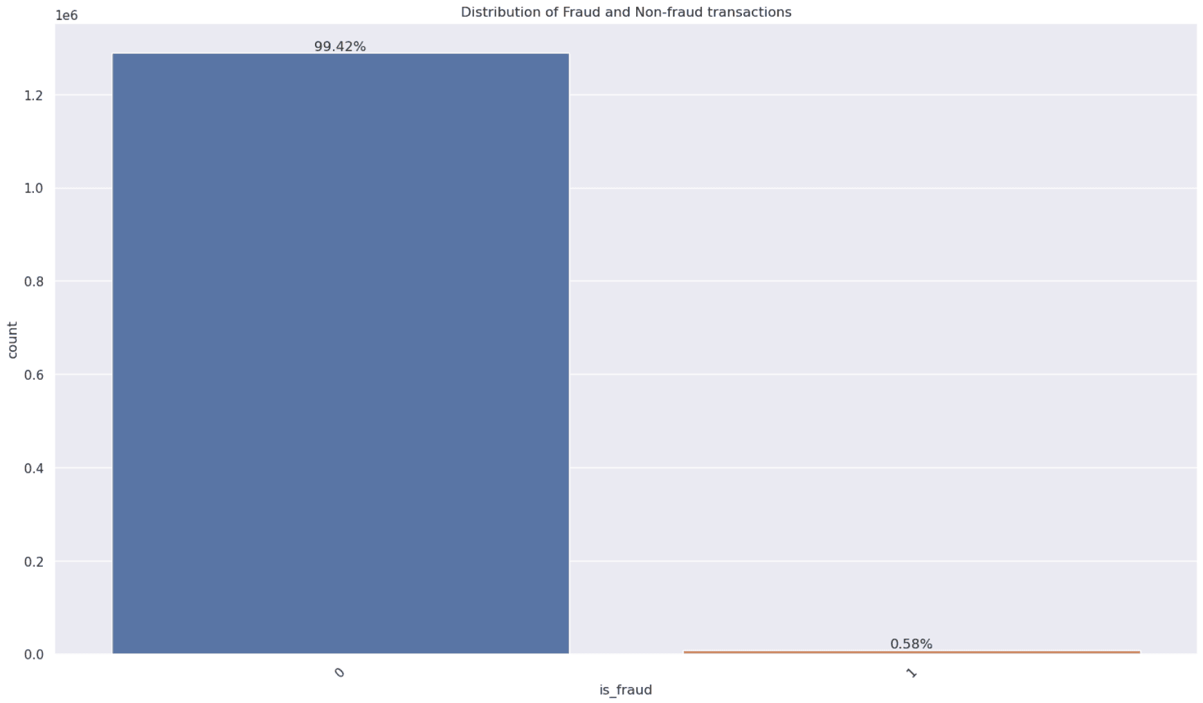
Based on the graph below, there are clearly far more non-fraud transactions than fraud transactions. A model trained on data this imbalanced can score highly just by predicting "not fraud" almost every time, so it may never learn to spot fraud properly. Balancing the classes is one way to fix this - this is where undersampling and oversampling come in later.
plot_graph(bank_data, 'is_fraud', "Distribution of Fraud and Non-fraud transactions", None)
plot_graph(bank_data, 'is_fraud', "Distribution of Fraud and Non-fraud transactions", None)
2. Do fraud transactions transfer more money than non-fraud transactions?
Plotting the amount spent for fraud and non-fraud transactions in a histogram reinforces the fact that the dataset has a very skewed distribution (as shown on the left histogram), but it also shows us that fraud transactions do not necessarily transfer more money than non-fraud transactions (as shown on the right histogram).
# Plotting amount spent for fraud and non-fraud transactions in a histogram
fig1, (ax1, ax2) = plt.subplots(nrows=1,ncols=2,figsize=(16,6))  # create set of subplots
plt.subplots_adjust(wspace=0.15)  # adjust space between matrixes so they don't overlap

for axes in (ax1, ax2):
    if axes==ax1:
        axes.hist(bank_data.loc[bank_data.is_fraud==0].amt, label='not fraud', bins=200, alpha=0.5)
        axes.set_ylabel("Count")
        axes.set_title("Amount Transferred against Fraud")
    if axes==ax2:
        axes.hist(bank_data.loc[bank_data.is_fraud==0].amt, label='not fraud', bins=1000, alpha=0.5)
        axes.set_ylim(0, 1200)
        axes.set_xlim(0, 2000)
        axes.set_title("Zoomed in - Amount Transferred against Fraud")
    axes.hist(bank_data.loc[bank_data.is_fraud==1].amt, label='fraud', bins=100, alpha=0.5)
    axes.set_xlabel("Amount transferred")
    axes.legend(['not fraud', 'fraud'])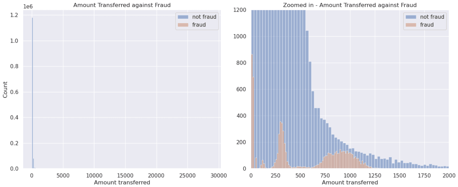
# Plotting amount spent for fraud and non-fraud transactions in a histogram
fig1, (ax1, ax2) = plt.subplots(nrows=1,ncols=2,figsize=(16,6))  # create set of subplots
plt.subplots_adjust(wspace=0.15)  # adjust space between matrixes so they don't overlap

for axes in (ax1, ax2):
    if axes==ax1:
        axes.hist(bank_data.loc[bank_data.is_fraud==0].amt, label='not fraud', bins=200, alpha=0.5)
        axes.set_ylabel("Count")
        axes.set_title("Amount Transferred against Fraud")
    if axes==ax2:
        axes.hist(bank_data.loc[bank_data.is_fraud==0].amt, label='not fraud', bins=1000, alpha=0.5)
        axes.set_ylim(0, 1200)
        axes.set_xlim(0, 2000)
        axes.set_title("Zoomed in - Amount Transferred against Fraud")
    axes.hist(bank_data.loc[bank_data.is_fraud==1].amt, label='fraud', bins=100, alpha=0.5)
    axes.set_xlabel("Amount transferred")
axes.legend(['not fraud', 'fraud'])3. Do some transaction categories involve more money being transferred than others?
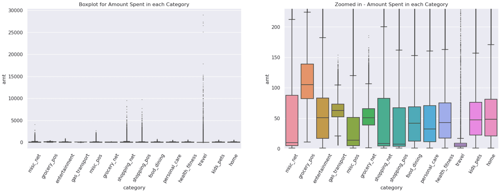
We can draw a box plot to investigate this - in most categories, there is a positive skew, so we would make the conclusion that in most categories, the transactions normally do not involve large amounts, but that there are a few especially large transactions taking place.
print("Maximum value of bank transaction:", bank_data["amt"].max())
print("Minimum value of bank transaction:", bank_data["amt"].min())

fig1, (ax1, ax2) = plt.subplots(nrows=1,ncols=2,figsize=(20,6))  # create set of subplots

sns.boxplot(data=bank_data,x="category",y="amt",ax=ax1,fliersize=0.5)
ax1.tick_params(axis='x',labelrotation=60)
ax1.set_title("Boxplot for Amount Spent in each Category")

sns.boxplot(data=bank_data,x="category",y="amt",ax=ax2, fliersize=0.5)
ax2.tick_params(axis='x',labelrotation=60)
plt.ylim(0,230)
ax2.set_title("Zoomed in - Amount Spent in each Category")
plt.show()
print("Maximum value of bank transaction:", bank_data["amt"].max())
print("Minimum value of bank transaction:", bank_data["amt"].min())

fig1, (ax1, ax2) = plt.subplots(nrows=1,ncols=2,figsize=(20,6))  # create set of subplots

sns.boxplot(data=bank_data,x="category",y="amt",ax=ax1,fliersize=0.5)
ax1.tick_params(axis='x',labelrotation=60)
ax1.set_title("Boxplot for Amount Spent in each Category")

sns.boxplot(data=bank_data,x="category",y="amt",ax=ax2, fliersize=0.5)
ax2.tick_params(axis='x',labelrotation=60)
plt.ylim(0,230)
ax2.set_title("Zoomed in - Amount Spent in each Category")
plt.show()
4. Do some transaction categories have a higher proportion of fraud transactions than others?
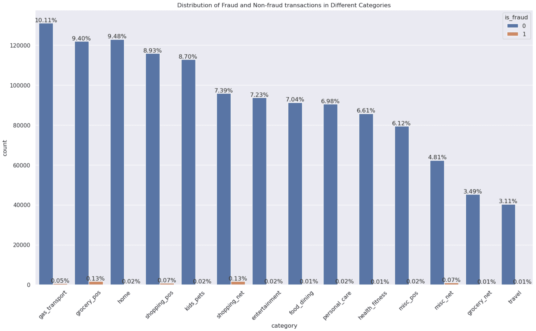
Outputting the distribution of fraud depending on categories shows us that all the categories contain some fraud transactions, however, groceries and shopping transactions have the most fraud transactions.
plot_graph(bank_data, 'category', "Distribution of Fraud and Non-fraud transactions in Different Categories", 'is_fraud')
plot_graph(bank_data, 'category', "Distribution of Fraud and Non-fraud transactions in Different Categories", 'is_fraud')
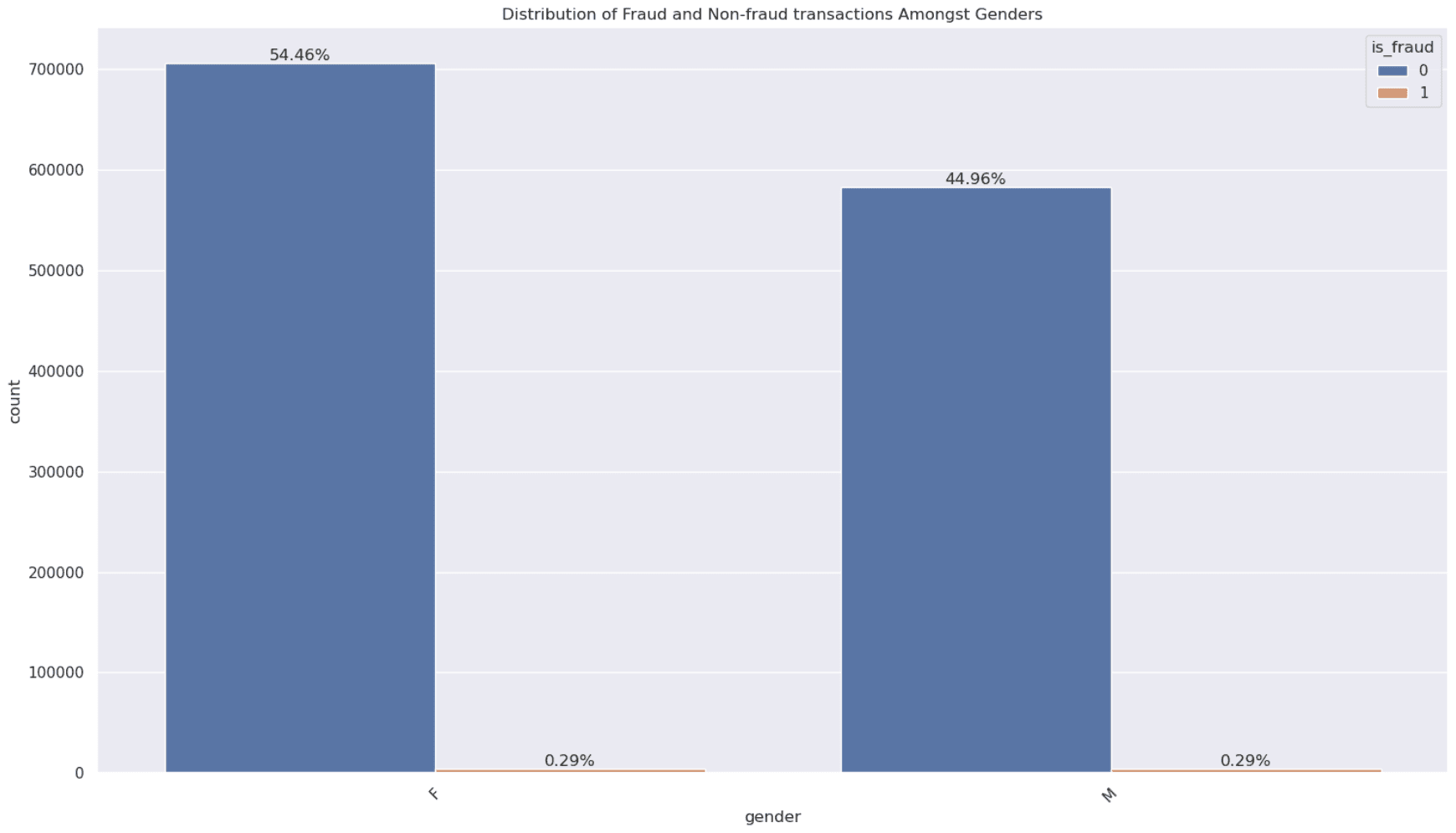
5. Does the gender of the person affect the proportion of fraud transactions that occur?
Both genders have an equal proportion of fraud transactions, but there are more bank transactions for females as opposed to males - gender doesn't seem to have a very large influence on fraud transactions.
plot_graph(bank_data, 'gender', "Distribution of Fraud and Non-fraud transactions Amongst Genders", 'is_fraud')
plot_graph(bank_data, 'gender', "Distribution of Fraud and Non-fraud transactions Amongst Genders", 'is_fraud')
6. Do some states have more fraud transactions than others? Does the total number of transactions in each state affect this?
TX, NY and PA have the highest proportion of transactions and similarly they also have the highest proportion of fraud transactions - with other states there also seems to be a strong positive correlation between the number of fraud transactions and total number of transactions.
fig1, (ax1, ax2) = plt.subplots(nrows=2,ncols=1,figsize=(35,20))  # create set of subplots
plt.subplots_adjust(hspace=0.2)  # adjust space between matrixes so they don't overlap

ax1.set_title("Distribution of Fraud and Non-fraud transactions in Different States")
plot1 = sns.countplot(bank_data, x='state', order=bank_data['state'].value_counts().index, hue='is_fraud', ax=ax1)
ax1.tick_params(axis='x',labelrotation=60)
fraud = bank_data[bank_data['is_fraud'] != 0]  # make a dataset that only contains fraud values.
ax2.set_title("Distribution of Fraud transactions in Different States")
plot2 = sns.countplot(fraud, x='state', order=fraud['state'].value_counts().index, hue=None, ax=ax2)
ax2.tick_params(axis='x',labelrotation=60)

for plot in (plot1,plot2):
    for bar in plot.containers:
        labels = [f'{h.get_height()/len(bank_data)*100:0.3f}%' for h in bar]
        plot.bar_label(bar, labels=labels, label_type='edge', rotation='vertical')
plt.show()
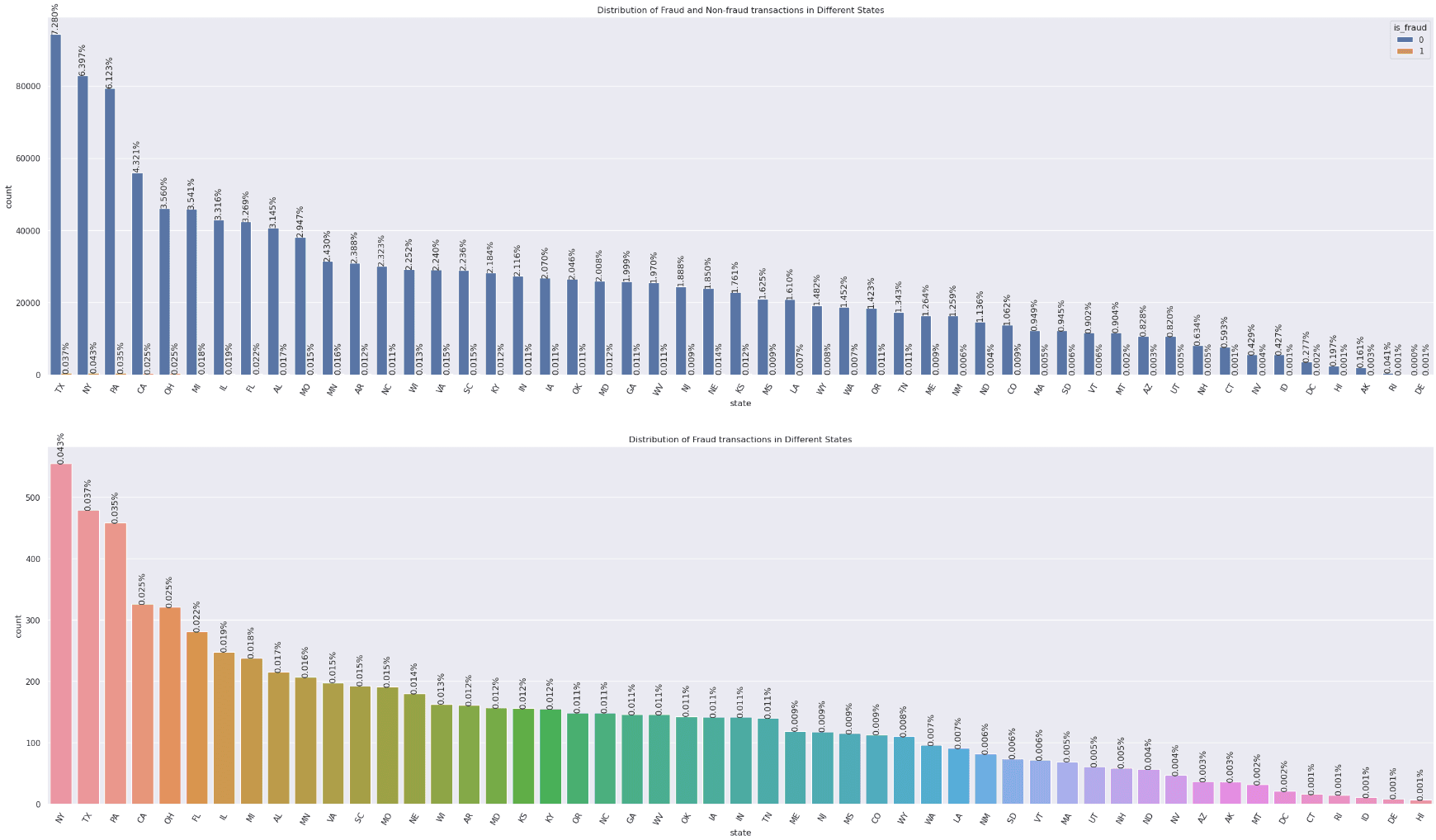
fig1, (ax1, ax2) = plt.subplots(nrows=2,ncols=1,figsize=(35,20))  # create set of subplots
plt.subplots_adjust(hspace=0.2)  # adjust space between matrixes so they don't overlap

ax1.set_title("Distribution of Fraud and Non-fraud transactions in Different States")
plot1 = sns.countplot(bank_data, x='state', order=bank_data['state'].value_counts().index, hue='is_fraud', ax=ax1)
ax1.tick_params(axis='x',labelrotation=60)
fraud = bank_data[bank_data['is_fraud'] != 0]  # make a dataset that only contains fraud values.
ax2.set_title("Distribution of Fraud transactions in Different States")
plot2 = sns.countplot(fraud, x='state', order=fraud['state'].value_counts().index, hue=None, ax=ax2)
ax2.tick_params(axis='x',labelrotation=60)

for plot in (plot1,plot2):
    for bar in plot.containers:
        labels = [f'{h.get_height()/len(bank_data)*100:0.3f}%' for h in bar]
        plot.bar_label(bar, labels=labels, label_type='edge', rotation='vertical')
plt.show()
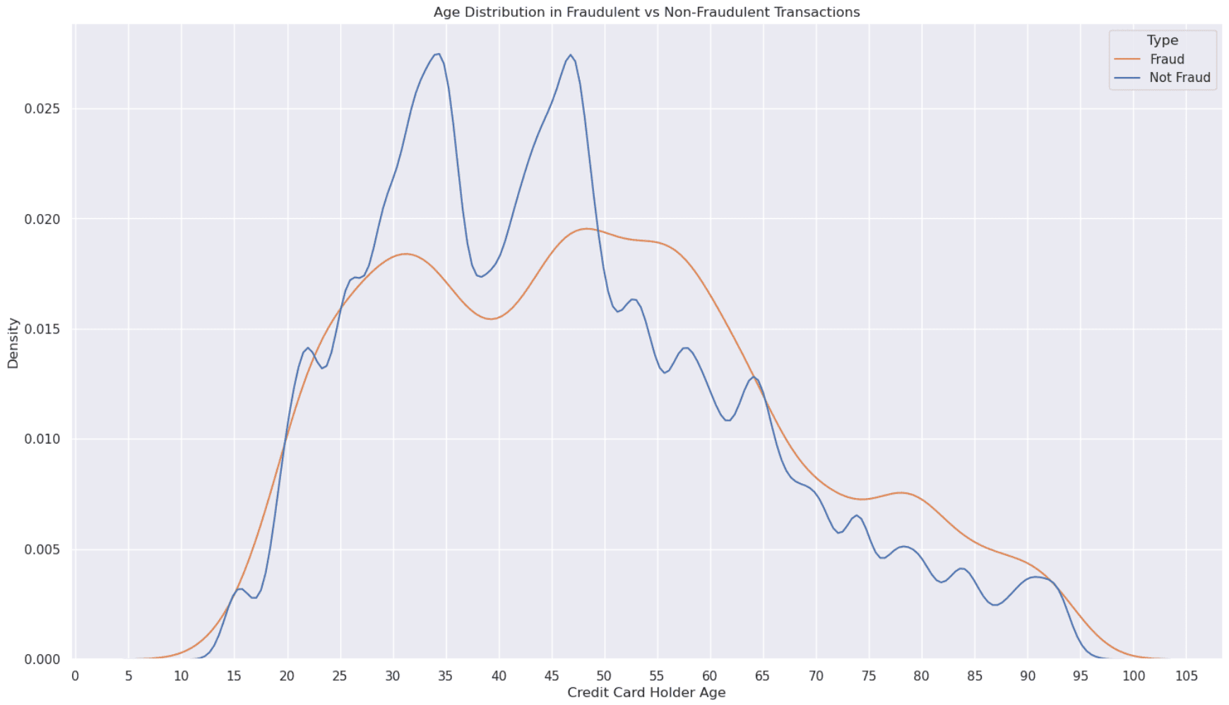
7. Are particular age groups more vulnerable to fraud transactions than others?
We can create a new feature in the dataset titled 'age' which calculates the age of the person at the time of the transaction: this is calculated by subtracting the person's date of birth from the transaction date.
The elderly population was not more prone to fraud transactions in this dataset: the most fraud transactions occured in the younger-middle age category, between people of ages 25 and 60 years old - this is also where the most normal transactions take place so it makes sense.
bank_data['age'] = pd.to_datetime(bank_data['trans_date_trans_time']).dt.year - pd.to_datetime(bank_data['dob']).dt.year
plt.figure(figsize=(18,10))
ax = sns.kdeplot(x='age',data=bank_data, hue='is_fraud', common_norm=False)
ax.set_xlabel('Credit Card Holder Age')
ax.set_ylabel('Density')
plt.xticks(np.arange(0,110,5))
plt.title('Age Distribution in Fraudulent vs Non-Fraudulent Transactions')
plt.legend(title='Type', labels=['Fraud', 'Not Fraud'])
plt.show()
bank_data['age'] = pd.to_datetime(bank_data['trans_date_trans_time']).dt.year - pd.to_datetime(bank_data['dob']).dt.year
plt.figure(figsize=(18,10))
ax = sns.kdeplot(x='age',data=bank_data, hue='is_fraud', common_norm=False)
ax.set_xlabel('Credit Card Holder Age')
ax.set_ylabel('Density')
plt.xticks(np.arange(0,110,5))
plt.title('Age Distribution in Fraudulent vs Non-Fraudulent Transactions')
plt.legend(title='Type', labels=['Fraud', 'Not Fraud'])
plt.show()
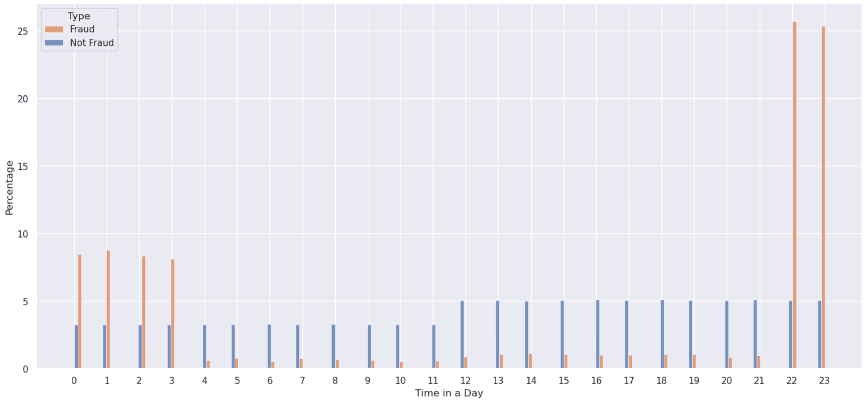
8. Do fraud transactions tend to occur at a particular time of the day?
Whilst most normal transactions occur regularly throughout the day, fraud transactions normally happen between 22:00 and 03:00 (when most people are asleep).
bank_data['hour'] = pd.to_datetime(bank_data['trans_date_trans_time']).dt.hour
plt.figure(figsize=(18,8))
ax = sns.histplot(data=bank_data, x="hour", hue="is_fraud", common_norm=False,stat='percent',multiple='dodge')
ax.set_ylabel('Percentage')
ax.set_xlabel('Time in a Day')
plt.xticks(np.arange(0,24,1))
plt.legend(title='Type', labels=['Fraud', 'Not Fraud'])
plt.show()
bank_data['hour'] = pd.to_datetime(bank_data['trans_date_trans_time']).dt.hour
plt.figure(figsize=(18,8))
ax = sns.histplot(data=bank_data, x="hour", hue="is_fraud", common_norm=False,stat='percent',multiple='dodge')
ax.set_ylabel('Percentage')
ax.set_xlabel('Time in a Day')
plt.xticks(np.arange(0,24,1))
plt.legend(title='Type', labels=['Fraud', 'Not Fraud'])
plt.show()
9. Do fraud transactions tend to occur at a particular day of the week?
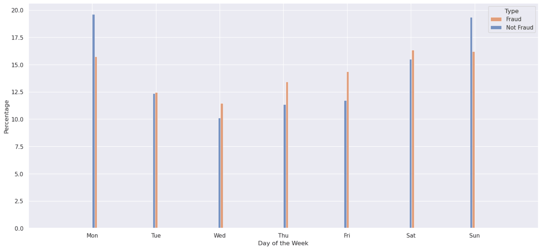
In general, fraud transactions are more prevalent on the weekend and Monday than during most weekdays - this mimics how more normal transactions tend to take place on the weekend and Monday.
During the week, fraud makes up a larger share of transactions than it does at the weekend - probably because more people work during the week and so do not go shopping/book holidays, etc. as much, so there are fewer normal transactions.
bank_data['day'] = pd.to_datetime(bank_data['trans_date_trans_time']).dt.dayofweek
plt.figure(figsize=(18,8))
ax = sns.histplot(data=bank_data,x="day",hue="is_fraud",common_norm=False,stat='percent',multiple='dodge')
ax.set_ylabel('Percentage')
ax.set_xlabel('Day of the Week')
ax.set_xticks(ax.get_xticks().tolist())  # set x-axis tick positions so they do not move when we do set_xticklabels
ax.set_xticklabels(["","Mon","Tue","Wed","Thu","Fri","Sat","Sun",""])
plt.legend(title='Type', labels=['Fraud', 'Not Fraud'])
plt.show()
bank_data['day'] = pd.to_datetime(bank_data['trans_date_trans_time']).dt.dayofweek
plt.figure(figsize=(18,8))
ax = sns.histplot(data=bank_data,x="day",hue="is_fraud",common_norm=False,stat='percent',multiple='dodge')
ax.set_ylabel('Percentage')
ax.set_xlabel('Day of the Week')
ax.set_xticks(ax.get_xticks().tolist())  # set x-axis tick positions so they do not move when we do set_xticklabels
ax.set_xticklabels(["","Mon","Tue","Wed","Thu","Fri","Sat","Sun",""])
plt.legend(title='Type', labels=['Fraud', 'Not Fraud'])
plt.show()
10. Do fraud transactions tend to occur in a particular month of the year?
Most normal bank transactions are made during March-June and December (when people either go on vacation or buy presents for Easter and Christmas), however fraud transactions mainly occur in the first half of the year and subside in the second half of the year.
bank_data['month'] = pd.to_datetime(bank_data['trans_date_trans_time']).dt.month
plt.figure(figsize=(18,8))
ax = sns.histplot(data=bank_data, x="month", hue="is_fraud", common_norm=False,stat='percent',multiple='dodge')
ax.set_ylabel('Percentage')
ax.set_xlabel('Month')
plt.xticks(np.arange(1,13,1))
ax.set_xticklabels(["Jan","Feb","Mar","Apr","May","Jun","Jul",'Aug','Sep','Oct','Nov','Dec'])
plt.legend(title='Type', labels=['Fraud', 'Not Fraud'])
plt.show()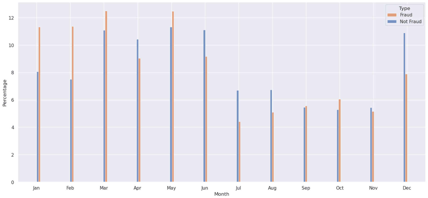
bank_data['month'] = pd.to_datetime(bank_data['trans_date_trans_time']).dt.month
plt.figure(figsize=(18,8))
ax = sns.histplot(data=bank_data, x="month", hue="is_fraud", common_norm=False,stat='percent',multiple='dodge')
ax.set_ylabel('Percentage')
ax.set_xlabel('Month')
plt.xticks(np.arange(1,13,1))
ax.set_xticklabels(["Jan","Feb","Mar","Apr","May","Jun","Jul",'Aug','Sep','Oct','Nov','Dec'])
plt.legend(title='Type', labels=['Fraud', 'Not Fraud'])
plt.show()Data Preprocessing
Feature Engineering and Selection
Feature engineering is creating, combining or transforming features to make them more useful to a model - like the age, hour, day and month features we built during the EDA. Feature selection is removing features that are irrelevant or not needed.
Printing out the number of unique values in each column shows us all the feature columns contain some variation that could help the ML models to differentiate between fraud and non-fraud transactions, so none seem to be irrelevant.
print("Number of unique values in each column:")
for x in list(bank_data.columns.values):
    print(x + ":", bank_data[x].nunique())
print("Number of unique values in each column:")
for x in list(bank_data.columns.values):
    print(x + ":", bank_data[x].nunique())
However, because the features 'first' and 'last' essentially just make up a full name, we can merge the two columns together, so that there are fewer features to process in total.
It's worth being cautious about keeping a name at all, though. A person's name shouldn't have anything to do with whether a transaction is fraudulent - it mostly acts as an ID for the cardholder, so a model can end up memorising which names appeared in fraud cases in the training data instead of learning general patterns. Dropping the name entirely would be a reasonable alternative, and a good experiment to compare against.
bank_data = bank_data.drop(labels=['trans_date_trans_time'], axis=1)
bank_data.head(5)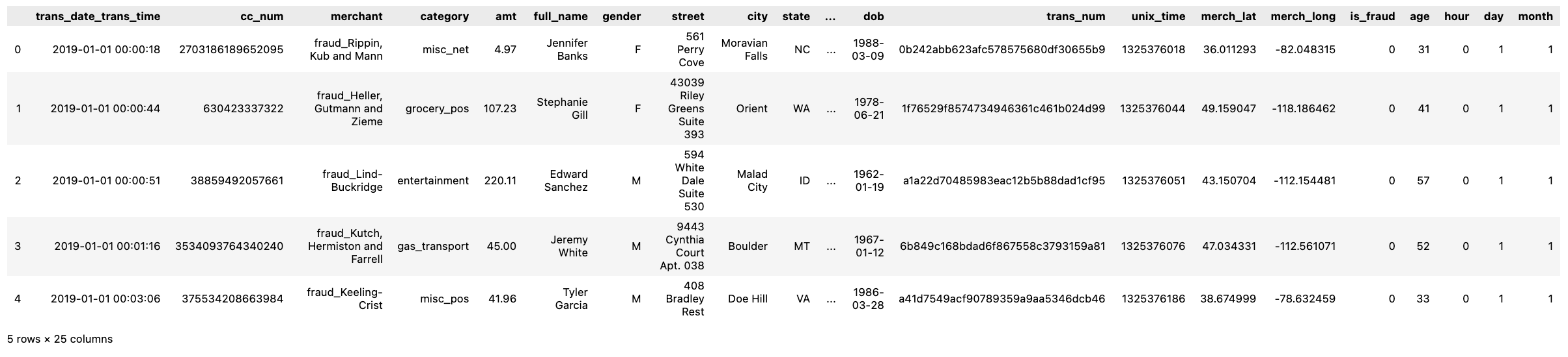
bank_data = bank_data.drop(labels=['trans_date_trans_time'], axis=1)
bank_data.head(5)We can also remove the column 'trans_date_trans_time' because it records the same information as 'unix_time' in a different format, and we've already processed it into hours, days, and months in our EDA.
col_categorical = bank_data.select_dtypes(include=['object']).columns
for col in col_categorical:
    bank_data[col] = bank_data[col].astype("category")
bank_data[col_categorical] = bank_data[col_categorical].apply(lambda x:x.cat.codes)
bank_data.head(5)
col_categorical = bank_data.select_dtypes(include=['object']).columns
for col in col_categorical:
    bank_data[col] = bank_data[col].astype("category")
bank_data[col_categorical] = bank_data[col_categorical].apply(lambda x:x.cat.codes)
bank_data.head(5)Categorical Encoding
Categorical encoding is converting the categories, merchant IDs and customer IDs into an integer format - it's needed in order to facilitate processing the data and performing undersampling and oversampling.
features = bank_data.drop(['is_fraud'], axis=1)
labels = bank_data['is_fraud']
features = bank_data.drop(['is_fraud'], axis=1)
labels = bank_data['is_fraud']Undersampling and Oversampling
Undersampling is when data from the majority class is removed from the dataset to balance it out, and oversampling is when more data of the minority class is added to the dataset to balance it out. Here we'll try both, and see which is more accurate.
We first need to divide the dataset into the features (e.g. cc_num, merchant, category, amt, full_name, gender, street) and the labels (i.e. is_fraud).
To control randomness, we can create a constant for the random seed so that we get reproducible results each time we run the ML models.
RANDOM_SEED = 2
tf.random.set_seed(RANDOM_SEED) # set random seed in tensorflow to 2RANDOM_SEED = 2
tf.random.set_seed(RANDOM_SEED) # set random seed in tensorflow to 2Undersampling:
rus = RandomUnderSampler(sampling_strategy='majority', random_state=RANDOM_SEED)
under_features, under_labels = rus.fit_resample(features, labels)
# We can print out the labels to see whether there are equal numbers of fraud and non-fraud transactions
print(under_labels.value_counts())0 7506 1 7506 Name: is_fraud, dtype: int64
rus = RandomUnderSampler(sampling_strategy='majority', random_state=RANDOM_SEED)
under_features, under_labels = rus.fit_resample(features, labels)
# We can print out the labels to see whether there are equal numbers of fraud and non-fraud transactions
print(under_labels.value_counts())0 7506 1 7506 Name: is_fraud, dtype: int64
Oversampling:
sm = SMOTE(random_state=RANDOM_SEED)
over_features, over_labels = sm.fit_resample(features,labels)
# We can print out the labels again to check there are equal numbers of fraud and non-fraud transactions
print(over_labels.value_counts())0 1289169 1 1289169 Name: is_fraud, dtype: int64
sm = SMOTE(random_state=RANDOM_SEED)
over_features, over_labels = sm.fit_resample(features,labels)
# We can print out the labels again to check there are equal numbers of fraud and non-fraud transactions
print(over_labels.value_counts())0 1289169 1 1289169 Name: is_fraud, dtype: int64
Feature Scaling
Feature scaling is a technique for rescaling all the independent features in a dataset to the same scale - K-Nearest Neighbours, Neural Networks and Logistic Regression all need this to function well. Standardisation is a type of feature scaling where each feature is rescaled so that its mean is 0 and its standard deviation is 1: this is what we will be using in this project.
col_names = features.columns  # create a list of the datasets' column names

s_scaler = StandardScaler()

under_ssfeatures = s_scaler.fit_transform(under_features)   # undersampled dataset converted to standardised numpy.ndarray
under_ssfeatures = pd.DataFrame(under_ssfeatures, columns=col_names)   # convert numpy.ndarray into a dataframe

over_ssfeatures = s_scaler.fit_transform(over_features)   # oversampled dataset
over_ssfeatures = pd.DataFrame(over_ssfeatures, columns=col_names)col_names = features.columns # create a list of the datasets' column names
s_scaler = StandardScaler()
under_ssfeatures = s_scaler.fit_transform(under_features) # undersampled dataset converted to standardised numpy.ndarray
under_ssfeatures = pd.DataFrame(under_ssfeatures, columns=col_names) # convert numpy.ndarray into a dataframe
over_ssfeatures = s_scaler.fit_transform(over_features) # oversampled dataset
over_ssfeatures = pd.DataFrame(over_ssfeatures, columns=col_names)Formatting the Test Dataset
The testing dataset needs to go through exactly the same preprocessing as the training dataset - the same cleaning, feature changes and encoding - otherwise the models would be tested on data in a different format from what they learned on. Ideally, the scaler should also be fitted on the training data only and then reused to transform the testing data, so that no information from the testing data leaks into training.
# Create pandas dataframe and read first 10 rows of the testing data.
test_data = pd.read_csv('../data/fraudTest.csv',usecols=range(1,23))
test_data.head(5)
# Create pandas dataframe and read first 10 rows of the testing data.
test_data = pd.read_csv('../data/fraudTest.csv',usecols=range(1,23))
test_data.head(5)# Feature engineering
# Merge the columns 'first' and 'last' into 'full_name'
test_data.insert(5, column='full_name', value=test_data[['first','last']].agg(' '.join, axis=1))
test_data = test_data.drop(labels=['first', 'last'], axis=1)
test_data.head(5)
# Feature engineering
# Merge the columns 'first' and 'last' into 'full_name'
test_data.insert(5, column='full_name', value=test_data[['first','last']].agg(' '.join, axis=1))
test_data = test_data.drop(labels=['first', 'last'], axis=1)
test_data.head(5)# Add all extra features added to the training dataset - must be in same order as training data for models to work
test_data['age'] = pd.to_datetime(test_data['trans_date_trans_time']).dt.year - pd.to_datetime(test_data['dob']).dt.year
test_data['hour'] = pd.to_datetime(test_data['trans_date_trans_time']).dt.hour
test_data['day'] = pd.to_datetime(test_data['trans_date_trans_time']).dt.dayofweek
test_data['month'] = pd.to_datetime(test_data['trans_date_trans_time']).dt.month# Add all extra features added to the training dataset - must be in same order as training data for models to work
test_data['age'] = pd.to_datetime(test_data['trans_date_trans_time']).dt.year - pd.to_datetime(test_data['dob']).dt.year
test_data['hour'] = pd.to_datetime(test_data['trans_date_trans_time']).dt.hour
test_data['day'] = pd.to_datetime(test_data['trans_date_trans_time']).dt.dayofweek
test_data['month'] = pd.to_datetime(test_data['trans_date_trans_time']).dt.month# Remove the feature 'trans_date_trans_time' because 'unix_time' is more accurate
test_data = test_data.drop(labels=['trans_date_trans_time'], axis=1)
test_data.head(5)
# Remove the feature 'trans_date_trans_time' because 'unix_time' is more accurate
test_data = test_data.drop(labels=['trans_date_trans_time'], axis=1)
test_data.head(5)# Category Encoding - convert feature columns to integer values - easier to process by ML models
col_categorical = test_data.select_dtypes(include=['object']).columns
for col in col_categorical:
test_data[col] = test_data[col].astype("category")
test_data[col_categorical] = test_data[col_categorical].apply(lambda x:x.cat.codes)
test_data.head(5)
# Category Encoding - convert feature columns to integer values - easier to process by ML models
col_categorical = test_data.select_dtypes(include=['object']).columns
for col in col_categorical:
    test_data[col] = test_data[col].astype("category")
test_data[col_categorical] = test_data[col_categorical].apply(lambda x:x.cat.codes)
test_data.head(5)# Divide test data into its features and labels
test_features = test_data.drop(['is_fraud'], axis=1)
test_labels = test_data['is_fraud']
test_labels.value_counts()0 553574 1 2145 Name: is_fraud, dtype: int64
# Divide test data into its features and labels
test_features = test_data.drop(['is_fraud'], axis=1)
test_labels = test_data['is_fraud']
test_labels.value_counts()0 553574 1 2145 Name: is_fraud, dtype: int64
# Feature scaling
test_ssfeatures = s_scaler.fit_transform(test_features)
test_ssfeatures = pd.DataFrame(test_ssfeatures, columns=col_names)# Feature scaling
test_ssfeatures = s_scaler.fit_transform(test_features)
test_ssfeatures = pd.DataFrame(test_ssfeatures, columns=col_names)Training and Testing the Models
We will output a classification report and 3 confusion matrices (one showing the proportion of values predicted, another showing the actual values and another showing the proportions of each class guessed correctly).
We can create our own function to plot the confusion matrices, because we will need to plot 3 for each model: '.subplots()' creates a figure and a set of subplots, which allows the confusion matrices to be shown side by side, and '.subplots_adjust()' makes sure they don't overlap. We use '.grid(False)' on each of the axes to remove the default grid lines, which would otherwise be drawn across the matrices.
def confusion_matrix_graph(test, prediction):
    fig1, (ax1, ax2, ax3) = plt.subplots(nrows=1,ncols=3,figsize=(12,8))  # create set of subplots
    plt.subplots_adjust(wspace=0.4)  # adjust space between matrixes so they don't overlap
    ax1.set_title("Actual values")  # add title
    ax1.grid(False)   # remove white lines
    disp1 = cmd.from_predictions(test, prediction, normalize=None, ax=ax1, colorbar=False) # removes colorbar
    plt.colorbar(disp1.im_,shrink=0.4)  # so we can add a new colorbar which is identical but smaller
    ax2.set_title("Proportions")  # as above
    ax2.grid(False)
    disp2 = cmd.from_predictions(test, prediction, normalize='all', ax=ax2, colorbar=False)
    plt.colorbar(disp2.im_,shrink=0.4)
    ax3.set_title("Class Proportions")
    ax3.grid(False)
    disp3 = cmd.from_predictions(test, prediction, normalize='true', ax=ax3, colorbar=False)
    plt.colorbar(disp3.im_,shrink=0.4)
plt.show() # show the plotsdef confusion_matrix_graph(test, prediction):
fig1, (ax1, ax2, ax3) = plt.subplots(nrows=1,ncols=3,figsize=(12,8)) # create set of subplots
plt.subplots_adjust(wspace=0.4) # adjust space between matrixes so they don't overlap
ax1.set_title("Actual values") # add title
ax1.grid(False) # remove white lines
disp1 = cmd.from_predictions(test, prediction, normalize=None, ax=ax1, colorbar=False) # removes colorbar
plt.colorbar(disp1.im_,shrink=0.4) # so we can add a new colorbar which is identical but smaller
ax2.set_title("Proportions") # as above
ax2.grid(False)
disp2 = cmd.from_predictions(test, prediction, normalize='all', ax=ax2, colorbar=False)
plt.colorbar(disp2.im_,shrink=0.4)
ax3.set_title("Class Proportions")
ax3.grid(False)
disp3 = cmd.from_predictions(test, prediction, normalize='true', ax=ax3, colorbar=False)
plt.colorbar(disp3.im_,shrink=0.4)
plt.show() # show the plotsKNN - Undersampled
start_time = time.time()  # get the current time and store this in the variable 'start_time'
uknn = KNeighborsClassifier(n_neighbors=25,p=2,weights='distance', n_jobs=-1,metric="euclidean")
uknn.fit(under_ssfeatures, under_labels)
uknn_pred = uknn.predict(test_ssfeatures)
print("Time taken: {} seconds".format(time.time()-start_time)) # subtract start_time from the current time to get running time of cell Time taken: 5.661163091659546 seconds
start_time = time.time()  # get the current time and store this in the variable 'start_time'
uknn = KNeighborsClassifier(n_neighbors=25,p=2,weights='distance', n_jobs=-1,metric="euclidean")
uknn.fit(under_ssfeatures, under_labels)
uknn_pred = uknn.predict(test_ssfeatures)
print("Time taken: {} seconds".format(time.time()-start_time)) # subtract start_time from the current time to get running time of cell Time taken: 5.661163091659546 seconds
print("Classification report for K Nearest Neighbors:\n", classification_report(test_labels, uknn_pred, digits=4))
print("\nConfusion matrices for K Nearest Neighbors:")
confusion_matrix_graph(test_labels, uknn_pred)Classification report for K Nearest Neighbors:
precision recall f1-score support
0 0.9988 0.7577 0.8617 553574
1 0.0122 0.7697 0.0239 2145
accuracy 0.7577 555719
macro avg 0.5055 0.7637 0.4428 555719
weighted avg 0.9950 0.7577 0.8585 555719
Confusion matrices for K Nearest Neighbors: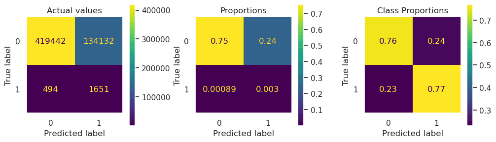
print("Classification report for K Nearest Neighbors:\n", classification_report(test_labels, uknn_pred, digits=4))
print("\nConfusion matrices for K Nearest Neighbors:")
confusion_matrix_graph(test_labels, uknn_pred)Classification report for K Nearest Neighbors:
precision recall f1-score support
0 0.9988 0.7577 0.8617 553574
1 0.0122 0.7697 0.0239 2145
accuracy 0.7577 555719
macro avg 0.5055 0.7637 0.4428 555719
weighted avg 0.9950 0.7577 0.8585 555719
Confusion matrices for K Nearest Neighbors:Its specificity and sensitivity are about equal. Its true negative and true positive rates are not as high as some models', and although its overall accuracy is reasonable, it flags a large share of normal transactions as fraud (a high false positive rate), which would make it impractical in real life.
KNN - Oversampled
start_time = time.time()  # get the current time and store this in the variable 'start_time'
oknn = KNeighborsClassifier(n_neighbors=75, p=2, n_jobs=-1)
oknn.fit(over_ssfeatures, over_labels)
oknn_pred = oknn.predict(test_ssfeatures)
print("Time taken: {} seconds".format(time.time()-start_time)) # subtract start_time from the current time to get running time of cell Time taken: 725.2192516326904 seconds
start_time = time.time()  # get the current time and store this in the variable 'start_time'
oknn = KNeighborsClassifier(n_neighbors=75, p=2, n_jobs=-1)
oknn.fit(over_ssfeatures, over_labels)
oknn_pred = oknn.predict(test_ssfeatures)
print("Time taken: {} seconds".format(time.time()-start_time)) # subtract start_time from the current time to get running time of cell Time taken: 725.2192516326904 seconds
print("Classification report for K Nearest Neighbors:\n", classification_report(test_labels, oknn_pred, digits=4))
print("\nConfusion matrices for K Nearest Neighbors:")
confusion_matrix_graph(test_labels, oknn_pred)Classification report for K Nearest Neighbors:
precision recall f1-score support
0 0.9976 0.8414 0.9129 553574
1 0.0116 0.4802 0.0226 2145
accuracy 0.8400 555719
macro avg 0.5046 0.6608 0.4678 555719
weighted avg 0.9938 0.8400 0.9094 555719
Confusion matrices for K Nearest Neighbors: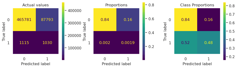
print("Classification report for K Nearest Neighbors:\n", classification_report(test_labels, oknn_pred, digits=4))
print("\nConfusion matrices for K Nearest Neighbors:")
confusion_matrix_graph(test_labels, oknn_pred)Classification report for K Nearest Neighbors:
precision recall f1-score support
0 0.9976 0.8414 0.9129 553574
1 0.0116 0.4802 0.0226 2145
accuracy 0.8400 555719
macro avg 0.5046 0.6608 0.4678 555719
weighted avg 0.9938 0.8400 0.9094 555719
Confusion matrices for K Nearest Neighbors:In contrast to the model which trained on the undersampled dataset, it has a much higher specificity than sensitivity. The model is far less accurate, however, so considering this and the very long runtime, this model wouldn't have any real life applications.
Random Forest - Undersampled
start_time = time.time()
urf_clf = RandomForestClassifier(n_estimators=100,max_depth=10,random_state=RANDOM_SEED,verbose=0,
                                 class_weight='balanced')
urf_clf.fit(under_features, under_labels)
urf_pred = urf_clf.predict(test_features)
print("Time taken: {} seconds".format(time.time()-start_time))Time taken: 6.661149740219116 seconds
start_time = time.time()
urf_clf = RandomForestClassifier(n_estimators=100,max_depth=10,random_state=RANDOM_SEED,verbose=0,
                                 class_weight='balanced')
urf_clf.fit(under_features, under_labels)
urf_pred = urf_clf.predict(test_features)
print("Time taken: {} seconds".format(time.time()-start_time))Time taken: 6.661149740219116 seconds
print("Classification report for RandomForestClassifier:\n", classification_report(test_labels, urf_pred, digits=4))
print("\nConfusion matrixes for RandomForestClassifier:")
confusion_matrix_graph(test_labels, urf_pred)Classification report for RandomForestClassifier:
precision recall f1-score support
0 0.9997 0.9671 0.9831 553574
1 0.0987 0.9296 0.1784 2145
accuracy 0.9670 555719
macro avg 0.5492 0.9484 0.5808 555719
weighted avg 0.9962 0.9670 0.9800 555719
Confusion matrixes for RandomForestClassifier: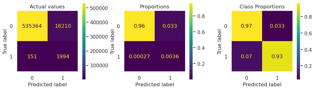
print("Classification report for RandomForestClassifier:\n", classification_report(test_labels, urf_pred, digits=4))
print("\nConfusion matrixes for RandomForestClassifier:")
confusion_matrix_graph(test_labels, urf_pred)Classification report for RandomForestClassifier:
precision recall f1-score support
0 0.9997 0.9671 0.9831 553574
1 0.0987 0.9296 0.1784 2145
accuracy 0.9670 555719
macro avg 0.5492 0.9484 0.5808 555719
weighted avg 0.9962 0.9670 0.9800 555719
Confusion matrixes for RandomForestClassifier:It is a good model as the true negative and true positive rates are very high - it has a high sensitivity and a high specificity, which is what we want. The runtime was also very low which is good - the algorithm is accurate and efficient, thus improving cost-effectiveness.
Random Forest - Oversampled
start_time = time.time()
orf_clf = RandomForestClassifier(n_estimators=100,max_depth=14,random_state=RANDOM_SEED,verbose=0,
                                 class_weight='balanced')
orf_clf.fit(over_features, over_labels)
orf_pred = orf_clf.predict(test_features)
print("Time taken: {} seconds".format(time.time()-start_time))Time taken: 686.8071060180664 seconds
start_time = time.time()
orf_clf = RandomForestClassifier(n_estimators=100,max_depth=14,random_state=RANDOM_SEED,verbose=0,
                                 class_weight='balanced')
orf_clf.fit(over_features, over_labels)
orf_pred = orf_clf.predict(test_features)
print("Time taken: {} seconds".format(time.time()-start_time))Time taken: 686.8071060180664 seconds
print("Classification report for RandomForestClassifier:\n", classification_report(test_labels, orf_pred, digits=4))
print("\nConfusion matrixes for RandomForestClassifier:")
confusion_matrix_graph(test_labels, orf_pred)Classification report for RandomForestClassifier:
precision recall f1-score support
0 0.9990 0.9846 0.9917 553574
1 0.1578 0.7450 0.2605 2145
accuracy 0.9837 555719
macro avg 0.5784 0.8648 0.6261 555719
weighted avg 0.9958 0.9837 0.9889 555719
Confusion matrixes for RandomForestClassifier: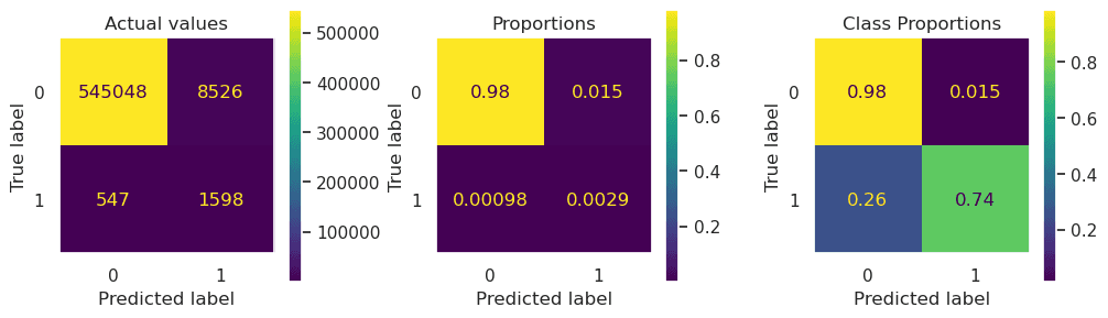
print("Classification report for RandomForestClassifier:\n", classification_report(test_labels, orf_pred, digits=4))
print("\nConfusion matrixes for RandomForestClassifier:")
confusion_matrix_graph(test_labels, orf_pred)Classification report for RandomForestClassifier:
precision recall f1-score support
0 0.9990 0.9846 0.9917 553574
1 0.1578 0.7450 0.2605 2145
accuracy 0.9837 555719
macro avg 0.5784 0.8648 0.6261 555719
weighted avg 0.9958 0.9837 0.9889 555719
Confusion matrixes for RandomForestClassifier:It didn't work as well as with the undersampled dataset. That's not too surprising: SMOTE doesn't add new information, it creates synthetic fraud examples by interpolating between existing ones, which can make a model overfit to the minority class. It still had both high specificity and high sensitivity (even if there is more specificity) so it is still a good model.
XGBoost - Undersampled
start_time = time.time()
uxgb_clf = xgb.XGBClassifier(learning_rate=0.05, n_estimators=400, objective='binary:hinge', n_jobs=-1,
                             nthread=None, base_score=0.5, random_state=RANDOM_SEED, verbosity=0)
uxgb_clf.fit(under_features, under_labels)
uxgb_pred = uxgb_clf.predict(test_features)
print("Time taken: {} seconds".format(time.time()-start_time))Time taken: 4.305298805236816 seconds
start_time = time.time()
uxgb_clf = xgb.XGBClassifier(learning_rate=0.05, n_estimators=400, objective='binary:hinge', n_jobs=-1,
                             nthread=None, base_score=0.5, random_state=RANDOM_SEED, verbosity=0)
uxgb_clf.fit(under_features, under_labels)
uxgb_pred = uxgb_clf.predict(test_features)
print("Time taken: {} seconds".format(time.time()-start_time))Time taken: 4.305298805236816 seconds
print("Classification report for XGBClassifier:\n", classification_report(test_labels, uxgb_pred, digits=4))
print("\nConfusion matrixes for XGBClassifier:")
confusion_matrix_graph(test_labels, uxgb_pred)Classification report for XGBClassifier:
precision recall f1-score support
0 0.9998 0.9755 0.9875 553574
1 0.1319 0.9594 0.2320 2145
accuracy 0.9755 555719
macro avg 0.5659 0.9675 0.6098 555719
weighted avg 0.9965 0.9755 0.9846 555719
Confusion matrixes for XGBClassifier: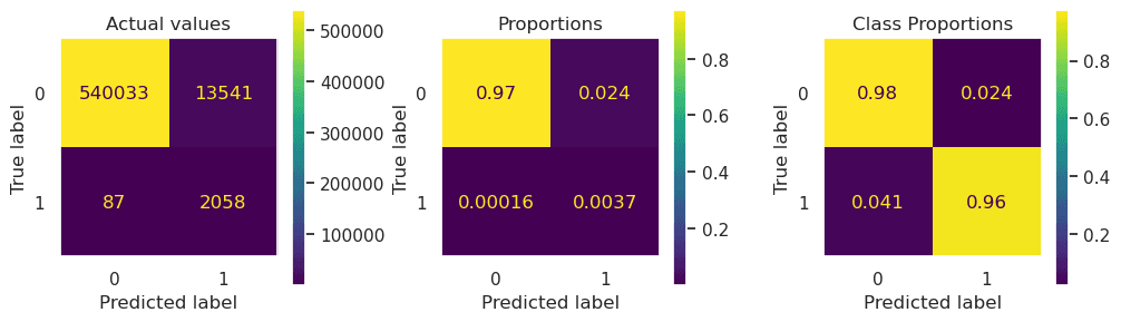
print("Classification report for XGBClassifier:\n", classification_report(test_labels, uxgb_pred, digits=4))
print("\nConfusion matrixes for XGBClassifier:")
confusion_matrix_graph(test_labels, uxgb_pred)Classification report for XGBClassifier:
precision recall f1-score support
0 0.9998 0.9755 0.9875 553574
1 0.1319 0.9594 0.2320 2145
accuracy 0.9755 555719
macro avg 0.5659 0.9675 0.6098 555719
weighted avg 0.9965 0.9755 0.9846 555719
Confusion matrixes for XGBClassifier:There is high specificity and sensitivity, which is good, so it seems to be very useful.
XGBoost - Oversampled
start_time = time.time()
oxgb_clf = xgb.XGBClassifier(learning_rate=0.05, n_estimators=400, objective='binary:hinge', n_jobs=-1,
                             nthread=None, base_score=0.5, random_state=RANDOM_SEED, verbosity=0)
oxgb_clf.fit(over_features, over_labels)
oxgb_pred = oxgb_clf.predict(test_features)
print("Time taken: {} seconds".format(time.time()-start_time))Time taken: 526.5862946510315 seconds
start_time = time.time()
oxgb_clf = xgb.XGBClassifier(learning_rate=0.05, n_estimators=400, objective='binary:hinge', n_jobs=-1,
                             nthread=None, base_score=0.5, random_state=RANDOM_SEED, verbosity=0)
oxgb_clf.fit(over_features, over_labels)
oxgb_pred = oxgb_clf.predict(test_features)
print("Time taken: {} seconds".format(time.time()-start_time))Time taken: 526.5862946510315 seconds
print("Classification report for XGBClassifier:\n", classification_report(test_labels, oxgb_pred, digits=4))
print("\nConfusion matrixes for XGBClassifier:")
confusion_matrix_graph(test_labels, oxgb_pred)Classification report for XGBClassifier:
precision recall f1-score support
0 0.9969 0.9977 0.9973 553574
1 0.2618 0.2121 0.2344 2145
accuracy 0.9947 555719
macro avg 0.6294 0.6049 0.6158 555719
weighted avg 0.9941 0.9947 0.9944 555719
Confusion matrixes for XGBClassifier: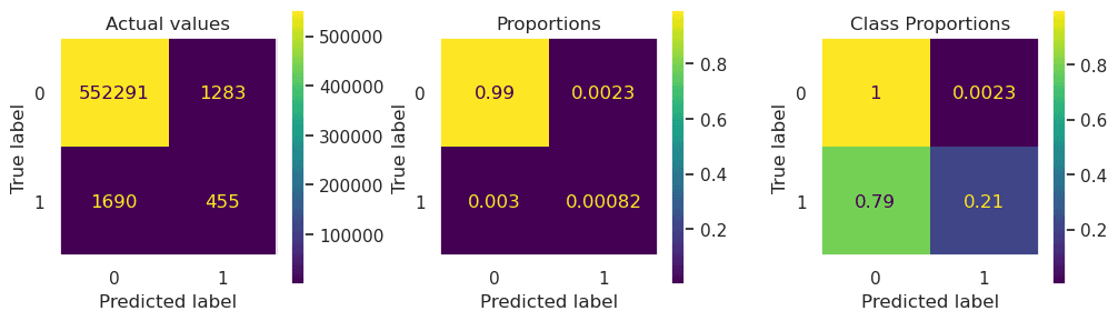
print("Classification report for XGBClassifier:\n", classification_report(test_labels, oxgb_pred, digits=4))
print("\nConfusion matrixes for XGBClassifier:")
confusion_matrix_graph(test_labels, oxgb_pred)Classification report for XGBClassifier:
precision recall f1-score support
0 0.9969 0.9977 0.9973 553574
1 0.2618 0.2121 0.2344 2145
accuracy 0.9947 555719
macro avg 0.6294 0.6049 0.6158 555719
weighted avg 0.9941 0.9947 0.9944 555719
Confusion matrixes for XGBClassifier:It didn't work as well as with the undersampled dataset - its specificity is outstanding but its sensitivity is awful. The runtime is not too long, however it is longer than some of the other models which trained on the oversampled dataset.
Logistic Regression - Undersampled
start_time = time.time()
ulr = LogisticRegression(solver='sag',penalty='l2',random_state=RANDOM_SEED)
ulr.fit(under_ssfeatures, under_labels)
ulr_pred = ulr.predict(test_ssfeatures)
print("Time taken: {} seconds".format(time.time()-start_time))Time taken: 0.33194875717163086 seconds
start_time = time.time()
ulr = LogisticRegression(solver='sag',penalty='l2',random_state=RANDOM_SEED)
ulr.fit(under_ssfeatures, under_labels)
ulr_pred = ulr.predict(test_ssfeatures)
print("Time taken: {} seconds".format(time.time()-start_time))Time taken: 0.33194875717163086 seconds
print("Classification report for LogisticRegression:\n", classification_report(test_labels, ulr_pred, digits=4))
print("\nConfusion matrixes for LogisticRegression:")
confusion_matrix_graph(test_labels, ulr_pred)Classification report for LogisticRegression:
precision recall f1-score support
0 0.9985 0.3988 0.5700 553574
1 0.0054 0.8462 0.0108 2145
accuracy 0.4005 555719
macro avg 0.5020 0.6225 0.2904 555719
weighted avg 0.9947 0.4005 0.5678 555719
Confusion matrixes for LogisticRegression: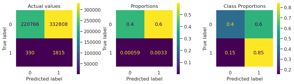
print("Classification report for LogisticRegression:\n", classification_report(test_labels, ulr_pred, digits=4))
print("\nConfusion matrixes for LogisticRegression:")
confusion_matrix_graph(test_labels, ulr_pred)Classification report for LogisticRegression:
precision recall f1-score support
0 0.9985 0.3988 0.5700 553574
1 0.0054 0.8462 0.0108 2145
accuracy 0.4005 555719
macro avg 0.5020 0.6225 0.2904 555719
weighted avg 0.9947 0.4005 0.5678 555719
Confusion matrixes for LogisticRegression:It has a very low specificity and a very high sensitivity: when predicting normal transactions, it is worse than a random classifier and when predicting fraud transactions it is quite accurate. Its runtime is very fast - although this does not make up for its inaccuracy, it does make it more efficient than other models such as KNN, which have a similar accuracy but a far longer runtime. However, its extremely low specificity means that it has few applications in real life.
Logistic Regression - Oversampled
start_time = time.time()
olr = LogisticRegression(solver='sag',penalty='l2',random_state=RANDOM_SEED)
olr.fit(over_ssfeatures, over_labels)
olr_pred = olr.predict(test_ssfeatures)
print("Time taken: {} seconds".format(time.time()-start_time))Time taken: 46.956894636154175 seconds
start_time = time.time()
olr = LogisticRegression(solver='sag',penalty='l2',random_state=RANDOM_SEED)
olr.fit(over_ssfeatures, over_labels)
olr_pred = olr.predict(test_ssfeatures)
print("Time taken: {} seconds".format(time.time()-start_time))Time taken: 46.956894636154175 seconds
print("Classification report for LogisticRegression:\n", classification_report(test_labels, olr_pred))
print("\nConfusion matrixes for LogisticRegression:")
confusion_matrix_graph(test_labels, olr_pred)Classification report for LogisticRegression:
precision recall f1-score support
0 1.00 0.38 0.55 553574
1 0.01 0.85 0.01 2145
accuracy 0.38 555719
macro avg 0.50 0.62 0.28 555719
weighted avg 0.99 0.38 0.55 555719
Confusion matrixes for LogisticRegression: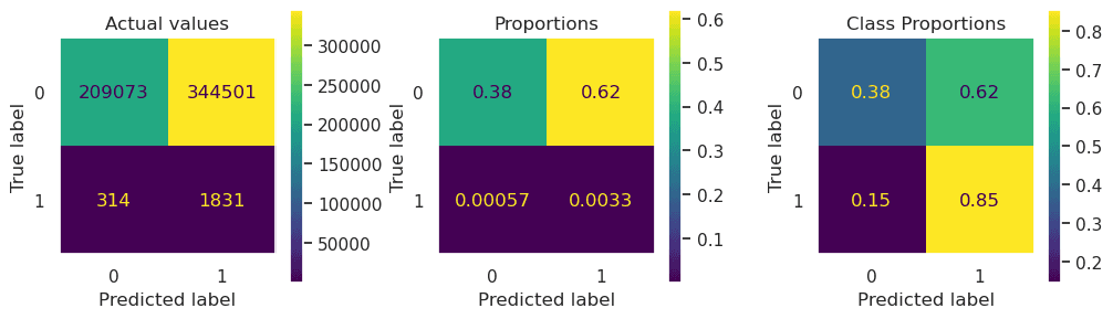
print("Classification report for LogisticRegression:\n", classification_report(test_labels, olr_pred))
print("\nConfusion matrixes for LogisticRegression:")
confusion_matrix_graph(test_labels, olr_pred)Classification report for LogisticRegression:
precision recall f1-score support
0 1.00 0.38 0.55 553574
1 0.01 0.85 0.01 2145
accuracy 0.38 555719
macro avg 0.50 0.62 0.28 555719
weighted avg 0.99 0.38 0.55 555719
Confusion matrixes for LogisticRegression:Similarly to the previous model, it has a very low specificity and a very high sensitivity. However, its extremely low specificity would mean that it would have very few applications in real life.
Neural Network - Undersampled
neural_network = tf.keras.Sequential([
    tf.keras.layers.Dense(units=30, input_dim=under_features.shape[1], activation='relu'),
    tf.keras.layers.Dropout(0.1),
    tf.keras.layers.Dense(units=35, activation='sigmoid'),
    tf.keras.layers.Dropout(0.1),
    tf.keras.layers.Dense(units=30, activation='sigmoid'),
    tf.keras.layers.Dropout(0.1),
    tf.keras.layers.Dense(units=20, activation='sigmoid'),
    tf.keras.layers.Dense(units=8, activation='sigmoid'),
    tf.keras.layers.Dense(units=1, activation='sigmoid')
])
neural_network.compile(loss='binary_crossentropy', optimizer='adam', metrics=['accuracy'])
early_stopping = tf.keras.callbacks.EarlyStopping(
    monitor='loss',verbose=1, patience=20, mode="min", restore_best_weights=True
)
neural_network.summary()Model: "sequential"
_________________________________________________________________
Layer (type) Output Shape Param #
=================================================================
dense (Dense) (None, 30) 720
dropout (Dropout) (None, 30) 0
dense_1 (Dense) (None, 35) 1085
dropout_1 (Dropout) (None, 35) 0
dense_2 (Dense) (None, 30) 1080
dropout_2 (Dropout) (None, 30) 0
dense_3 (Dense) (None, 20) 620
dense_4 (Dense) (None, 8) 168
dense_5 (Dense) (None, 1) 9
=================================================================
Total params: 3,682
Trainable params: 3,682
Non-trainable params: 0neural_network = tf.keras.Sequential([
tf.keras.layers.Dense(units=30, input_dim=under_features.shape[1], activation='relu'),
tf.keras.layers.Dropout(0.1),
tf.keras.layers.Dense(units=35, activation='sigmoid'),
tf.keras.layers.Dropout(0.1),
tf.keras.layers.Dense(units=30, activation='sigmoid'),
tf.keras.layers.Dropout(0.1),
tf.keras.layers.Dense(units=20, activation='sigmoid'),
tf.keras.layers.Dense(units=8, activation='sigmoid'),
tf.keras.layers.Dense(units=1, activation='sigmoid')
])
neural_network.compile(loss='binary_crossentropy', optimizer='adam', metrics=['accuracy'])
early_stopping = tf.keras.callbacks.EarlyStopping(
monitor='loss',verbose=1, patience=20, mode="min", restore_best_weights=True
)
neural_network.summary()Model: "sequential"
_________________________________________________________________
Layer (type) Output Shape Param #
=================================================================
dense (Dense) (None, 30) 720
dropout (Dropout) (None, 30) 0
dense_1 (Dense) (None, 35) 1085
dropout_1 (Dropout) (None, 35) 0
dense_2 (Dense) (None, 30) 1080
dropout_2 (Dropout) (None, 30) 0
dense_3 (Dense) (None, 20) 620
dense_4 (Dense) (None, 8) 168
dense_5 (Dense) (None, 1) 9
=================================================================
Total params: 3,682
Trainable params: 3,682
Non-trainable params: 0start_time = time.time()
neural_network.fit(under_ssfeatures, under_labels, epochs=500, batch_size=1000 , verbose=0, shuffle=True, callbacks=early_stopping)
unn_pred = neural_network.predict(test_ssfeatures) > 0.5
print("Time taken: {} seconds".format(time.time()-start_time))Restoring model weights from the end of the best epoch: 117. Epoch 137: early stopping 17367/17367 [==============================] - 12s 695us/step Time taken: 25.322855949401855 seconds
start_time = time.time()
neural_network.fit(under_ssfeatures, under_labels, epochs=500, batch_size=1000 , verbose=0, shuffle=True, callbacks=early_stopping)
unn_pred = neural_network.predict(test_ssfeatures) > 0.5
print("Time taken: {} seconds".format(time.time()-start_time))Restoring model weights from the end of the best epoch: 117. Epoch 137: early stopping 17367/17367 [==============================] - 12s 695us/step Time taken: 25.322855949401855 seconds
print("Classification report for Neural Network:\n", classification_report(test_labels, unn_pred, digits=4))
print("\nConfusion matrixes for Neural Network:")
confusion_matrix_graph(test_labels, unn_pred)Classification report for Neural Network:
precision recall f1-score support
0 0.9987 0.5651 0.7218 553574
1 0.0072 0.8145 0.0143 2145
accuracy 0.5661 555719
macro avg 0.5030 0.6898 0.3680 555719
weighted avg 0.9949 0.5661 0.7191 555719
Confusion matrixes for Neural Network: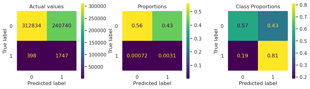
print("Classification report for Neural Network:\n", classification_report(test_labels, unn_pred, digits=4))
print("\nConfusion matrixes for Neural Network:")
confusion_matrix_graph(test_labels, unn_pred)Classification report for Neural Network:
precision recall f1-score support
0 0.9987 0.5651 0.7218 553574
1 0.0072 0.8145 0.0143 2145
accuracy 0.5661 555719
macro avg 0.5030 0.6898 0.3680 555719
weighted avg 0.9949 0.5661 0.7191 555719
Confusion matrixes for Neural Network:It has a very low specificity and a very high sensitivity: when predicting normal transactions, it is essentially a random classifier and when predicting fraud transactions it is very accurate. It is worth noting that it takes up a significant amount of processor time, and the low specificity means that it does not have many real life applications.
Neural Network - Oversampled
neural_network = tf.keras.Sequential([
    tf.keras.layers.Dense(units=100, input_dim=under_features.shape[1], activation='relu'),
    tf.keras.layers.Dropout(0.1),
    tf.keras.layers.Dense(units=70, activation='sigmoid'),
    tf.keras.layers.Dropout(0.1),
    tf.keras.layers.Dense(units=60, activation='sigmoid'),
    tf.keras.layers.Dropout(0.1),
    tf.keras.layers.Dense(units=50, activation='sigmoid'),
    tf.keras.layers.Dropout(0.1),
    tf.keras.layers.Dense(units=40, activation='sigmoid'),
    tf.keras.layers.Dropout(0.1),
    tf.keras.layers.Dense(units=40, activation='sigmoid'),
    tf.keras.layers.Dense(units=30, activation='sigmoid'),
    tf.keras.layers.Dense(units=20, activation='sigmoid'),
    tf.keras.layers.Dense(units=10, activation='sigmoid'),
    tf.keras.layers.Dense(units=8, activation='sigmoid'),
    tf.keras.layers.Dense(units=1, activation='sigmoid')
])
neural_network.compile(loss='binary_crossentropy', optimizer='adam', metrics=['accuracy'])
early_stopping = tf.keras.callbacks.EarlyStopping(
    monitor='loss',verbose=1, patience=20, mode="min", restore_best_weights=True
)
neural_network.summary()Model: "sequential_1"
_________________________________________________________________
Layer (type) Output Shape Param #
=================================================================
dense_6 (Dense) (None, 100) 2400
dropout_3 (Dropout) (None, 100) 0
dense_7 (Dense) (None, 70) 7070
dropout_4 (Dropout) (None, 70) 0
dense_8 (Dense) (None, 60) 4260
dropout_5 (Dropout) (None, 60) 0
dense_9 (Dense) (None, 50) 3050
dropout_6 (Dropout) (None, 50) 0
dense_10 (Dense) (None, 40) 2040
dropout_7 (Dropout) (None, 40) 0
dense_11 (Dense) (None, 40) 1640
...
Total params: 22,617
Trainable params: 22,617
Non-trainable params: 0neural_network = tf.keras.Sequential([
tf.keras.layers.Dense(units=100, input_dim=under_features.shape[1], activation='relu'),
tf.keras.layers.Dropout(0.1),
tf.keras.layers.Dense(units=70, activation='sigmoid'),
tf.keras.layers.Dropout(0.1),
tf.keras.layers.Dense(units=60, activation='sigmoid'),
tf.keras.layers.Dropout(0.1),
tf.keras.layers.Dense(units=50, activation='sigmoid'),
tf.keras.layers.Dropout(0.1),
tf.keras.layers.Dense(units=40, activation='sigmoid'),
tf.keras.layers.Dropout(0.1),
tf.keras.layers.Dense(units=40, activation='sigmoid'),
tf.keras.layers.Dense(units=30, activation='sigmoid'),
tf.keras.layers.Dense(units=20, activation='sigmoid'),
tf.keras.layers.Dense(units=10, activation='sigmoid'),
tf.keras.layers.Dense(units=8, activation='sigmoid'),
tf.keras.layers.Dense(units=1, activation='sigmoid')
])
neural_network.compile(loss='binary_crossentropy', optimizer='adam', metrics=['accuracy'])
early_stopping = tf.keras.callbacks.EarlyStopping(
monitor='loss',verbose=1, patience=20, mode="min", restore_best_weights=True
)
neural_network.summary()Model: "sequential_1"
_________________________________________________________________
Layer (type) Output Shape Param #
=================================================================
dense_6 (Dense) (None, 100) 2400
dropout_3 (Dropout) (None, 100) 0
dense_7 (Dense) (None, 70) 7070
dropout_4 (Dropout) (None, 70) 0
dense_8 (Dense) (None, 60) 4260
dropout_5 (Dropout) (None, 60) 0
dense_9 (Dense) (None, 50) 3050
dropout_6 (Dropout) (None, 50) 0
dense_10 (Dense) (None, 40) 2040
dropout_7 (Dropout) (None, 40) 0
dense_11 (Dense) (None, 40) 1640
...
Total params: 22,617
Trainable params: 22,617
Non-trainable params: 0start_time = time.time()
neural_network.fit(over_ssfeatures, over_labels, epochs=500, batch_size=2000 , verbose=0, shuffle=True, callbacks=early_stopping)
onn_pred = neural_network.predict(test_ssfeatures) > 0.5
print("Time taken: {} seconds".format(time.time()-start_time))Restoring model weights from the end of the best epoch: 402. Epoch 422: early stopping 17367/17367 [==============================] - 14s 818us/step Time taken: 4071.172511577606 seconds
start_time = time.time()
neural_network.fit(over_ssfeatures, over_labels, epochs=500, batch_size=2000 , verbose=0, shuffle=True, callbacks=early_stopping)
onn_pred = neural_network.predict(test_ssfeatures) > 0.5
print("Time taken: {} seconds".format(time.time()-start_time))Restoring model weights from the end of the best epoch: 402. Epoch 422: early stopping 17367/17367 [==============================] - 14s 818us/step Time taken: 4071.172511577606 seconds
print("Classification report for Neural Network:\n", classification_report(test_labels, onn_pred, digits=4))
print("\nConfusion matrixes for Neural Network:")
confusion_matrix_graph(test_labels, onn_pred)Classification report for Neural Network:
precision recall f1-score support
0 0.9956 0.6255 0.7683 553574
1 0.0030 0.2886 0.0059 2145
accuracy 0.6242 555719
macro avg 0.4993 0.4571 0.3871 555719
weighted avg 0.9918 0.6242 0.7654 555719
Confusion matrixes for Neural Network: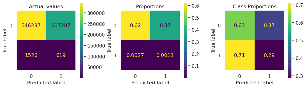
print("Classification report for Neural Network:\n", classification_report(test_labels, onn_pred, digits=4))
print("\nConfusion matrixes for Neural Network:")
confusion_matrix_graph(test_labels, onn_pred)Classification report for Neural Network:
precision recall f1-score support
0 0.9956 0.6255 0.7683 553574
1 0.0030 0.2886 0.0059 2145
accuracy 0.6242 555719
macro avg 0.4993 0.4571 0.3871 555719
weighted avg 0.9918 0.6242 0.7654 555719
Confusion matrixes for Neural Network:The sensitivity is moderately high whereas the specificity is very low - considering its inaccuracy and extremely long runtime, it doesn't seem to be useful.
Conclusions
To compare our models we'll use the ROC AUC: the Area Under the Receiver Operating Characteristic Curve.
The higher the AUC, the better. We can use this to compare the models overall, before analysing each of their true/false negative/positive rates to grasp which are more effective.
Firstly, we need a baseline to compare against. We'll make a list of predictions that consists only of one class ("not fraud"): this is a no-skill classifier with an AUC of 0.5, the same as random guessing, so any useful model should do better than it.
random_pred = [0 for i in range(len(test_labels))]random_pred = [0 for i in range(len(test_labels))]Now we'll use matplotlib and sklearn to create our own function that plots the ROC curves and their AUCs for us.
def plot_roc_auc(model, y_test, preds, color):
    # Takes actual and predicted (probabilities) as input and plots the curve
    fpr, tpr, threshold = roc_curve(y_test, preds)
    roc_auc = auc(fpr, tpr)
plt.plot(fpr, tpr, color, label = str(model + 'AUC = %0.2f' % roc_auc))def plot_roc_auc(model, y_test, preds, color):
# Takes actual and predicted (probabilities) as input and plots the curve
fpr, tpr, threshold = roc_curve(y_test, preds)
roc_auc = auc(fpr, tpr)
plt.plot(fpr, tpr, color, label = str(model + 'AUC = %0.2f' % roc_auc))plt.figure(figsize=(14,7))
plot_roc_auc('Random Classifier -> ', test_labels, random_pred, 'k')
plot_roc_auc("XGBoost -> ", test_labels, uxgb_pred, 'y')
plot_roc_auc("Random Forest -> ", test_labels, urf_pred, 'c')
plot_roc_auc("KNN -> ", test_labels, uknn_pred, 'm')
plot_roc_auc("Neural Network -> ", test_labels, unn_pred, 'g')
plot_roc_auc("Logistic Regression -> ", test_labels, ulr_pred, 'r')
plt.title('Undersampling - Receiver Operating Characteristic')
plt.legend(loc = 'lower right', fontsize=10)
plt.xlim([0, 1])
plt.ylim([0, 1])
plt.ylabel('True Positive Rate')
plt.xlabel('False Positive Rate')
plt.show()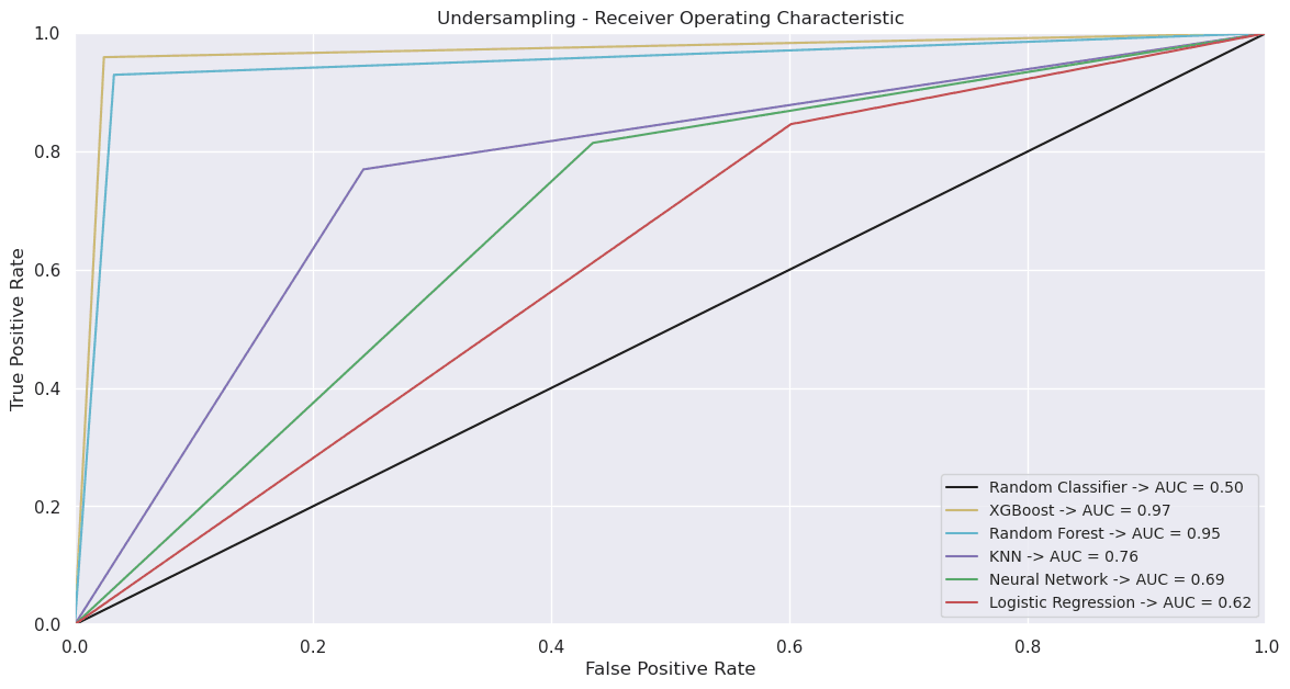
plt.figure(figsize=(14,7))
plot_roc_auc('Random Classifier -> ', test_labels, random_pred, 'k')
plot_roc_auc("XGBoost -> ", test_labels, uxgb_pred, 'y')
plot_roc_auc("Random Forest -> ", test_labels, urf_pred, 'c')
plot_roc_auc("KNN -> ", test_labels, uknn_pred, 'm')
plot_roc_auc("Neural Network -> ", test_labels, unn_pred, 'g')
plot_roc_auc("Logistic Regression -> ", test_labels, ulr_pred, 'r')

plt.title('Undersampling - Receiver Operating Characteristic')
plt.legend(loc = 'lower right', fontsize=10)
plt.xlim([0, 1])
plt.ylim([0, 1])
plt.ylabel('True Positive Rate')
plt.xlabel('False Positive Rate')
plt.show()Ranked by AUC, from best to worst, the models are: XGBoost, Random Forest, KNN, Neural Network and Logistic Regression. XGBoost and Random Forest also had the quickest runtimes, so out of all the models used, these were probably the best. KNN and the Neural Network had an adequate accuracy, however the long runtime is a significant drawback, and for Logistic Regression, the short runtime is not particularly useful if the accuracy is not as high.
plt.figure(figsize=(14,7))
plot_roc_auc('Random Classifier -> ', test_labels, random_pred, 'k')
plot_roc_auc("XGBoost -> ", test_labels, oxgb_pred, 'y')
plot_roc_auc("Random Forest -> ", test_labels, orf_pred, 'c')
plot_roc_auc("KNN -> ", test_labels, oknn_pred, 'm')
plot_roc_auc('Neural Network -> ', test_labels, onn_pred, 'g')
plot_roc_auc('Logistic Regression -> ', test_labels, olr_pred, 'r')

plt.title('Overersampling - Receiver Operating Characteristic')
plt.legend(loc = 'lower right', fontsize=10)
plt.plot([0, 1], [0, 1],'r--')
plt.xlim([0, 1])
plt.ylim([0, 1])
plt.ylabel('True Positive Rate')
plt.xlabel('False Positive Rate')
plt.show()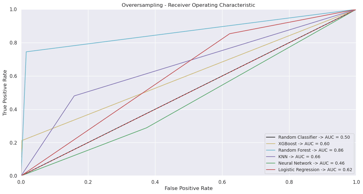
plt.figure(figsize=(14,7))
plot_roc_auc('Random Classifier -> ', test_labels, random_pred, 'k')
plot_roc_auc("XGBoost -> ", test_labels, oxgb_pred, 'y')
plot_roc_auc("Random Forest -> ", test_labels, orf_pred, 'c')
plot_roc_auc("KNN -> ", test_labels, oknn_pred, 'm')
plot_roc_auc('Neural Network -> ', test_labels, onn_pred, 'g')
plot_roc_auc('Logistic Regression -> ', test_labels, olr_pred, 'r')

plt.title('Overersampling - Receiver Operating Characteristic')
plt.legend(loc = 'lower right', fontsize=10)
plt.plot([0, 1], [0, 1],'r--')
plt.xlim([0, 1])
plt.ylim([0, 1])
plt.ylabel('True Positive Rate')
plt.xlabel('False Positive Rate')
plt.show()All of the models' AUCs decreased. It's tempting to expect the larger oversampled dataset to help, but the extra fraud examples are synthetic copies interpolated from the existing ones, so they add no new information and can lead the models to overfit. Random Forest was the best classifier this time, whereas KNN's and XGBoost's AUCs decreased dramatically (as can be seen with both the curve and the AUC).
Thanks for reading - I hope this helps, and don't forget to check out the full source code on GitHub too!